Tutorial: Multi-Energy refinement
It is often advantageous to refine reflectivity measured at multiple photon energies simultaneously in order to determine a unique model. The intrinsic contrast afforded at resonance allows for simple global fits for improved model uniqueness. This tutorial will present a suitable method to simultaneously refine datasets taken across multiple energies on a single sample.
Initialize PyPXR
We begin by initializing the same modules for fitting polarized reflectivity as stated in the first tutorial. The only new function required is GlobalObjective that will allow for simultaneous model refinement
[1]:
%matplotlib inline

import os.path
import sys
import numpy as np
import matplotlib.pyplot as plt
import h5py

sys.path.append("../../../src/PyPXR") # Temporary solution until hosted on pip

from reflectivity import *
from structure import *

# For Fitting
from refnx.dataset import ReflectDataset # Object used to define data
from refnx.analysis import Transform, CurveFitter, Objective, GlobalObjective
PyPXR provides two datasets for this example measured on the same sample
[2]:
mypath = "../../../src/PyPXR/example_data/"
# Energy 1 - 284.7 eV
data_spol_en1 = os.path.join(mypath, 'Feb19_Exp101_p100.txt')  # s-pol data
data_ppol_en1 = os.path.join(mypath, 'Feb19_Exp101_p190.txt')  # p-pol data
mydata_s1 = np.genfromtxt(data_spol_en1, delimiter='\t')
mydata_p1 = np.genfromtxt(data_ppol_en1, delimiter='\t')

# Energy 2 - 285.7 eV
data_spol_en2 = os.path.join(mypath, 'Feb19_Exp102_p100.txt')  # s-pol data
data_ppol_en2 = os.path.join(mypath, 'Feb19_Exp102_p190.txt')  # p-pol data
mydata_s2 = np.genfromtxt(data_spol_en2, delimiter='\t')
mydata_p2 = np.genfromtxt(data_ppol_en2, delimiter='\t')

# Concatenate spol / ppol data together for fitting
mydata_en1 = np.concatenate([mydata_s1, mydata_p1])
mydata_en2 = np.concatenate([mydata_s2, mydata_p2])

# Construct objects to use refnx fitting modules, a Transpose is called to set the axis correctly
data_en1 = ReflectDataset(mydata_en1.T)
data_en2 = ReflectDataset(mydata_en2.T)
To initiate multi-energy model refinement we will utilize a combination of two strategies:
Shared
PXR_Slabobjects that are identical between data-sets. Properties can be determined through an input energy.A series of inter-slab constraints that allow us to ensure identical structural parameters (thickness, roughness, etc.)
Create models for each dataset.
[3]:
# List of energies associated with each dataset
# en1 = 284.7 eV
# en2 = 285.7 ev
en_list = [284.7, 285.7] #[eV]

# Substrate / Superstrate objects
# These objects will be used in both structures
si = PXR_MaterialSLD('Si', density=2.33, name='Si') #Substrate
sio2 = PXR_MaterialSLD('SiO2', density=2.28, name='SiO2') #Substrate
vacuum = PXR_MaterialSLD('', density=1, name='vacuum') #Superstrate

# Slabs for each material
si_slab = si(0, 0.5) #thickness of bounding substrate does not matter
sio2_slab = sio2(12, 1)
We did not specify a photon energy for these PXR_MaterialSLD items. When we call PXR_ReflectModel it will update the structure based on the input energy. This allows us to use a single slab object for both structures.
Build energy-dependent structure components
We now want to craft four PXR_SLD objects (2 layers x 2 energies) with uniaxial optical parameters.
[4]:
# Energy 1
# Bulk object
n_xx1 = complex(-0.00043, 0.0001) # [unitless] #Ordinary Axis
n_zz1 = complex(-0.00049, 0.00019) # [unitless] #Extraordinary Axis
posa_en1 = PXR_SLD(np.array([n_xx1, n_zz1]), name='posa1') #Molecule
# Surface objet
n_xx1 = complex(-0.00019, 0.00152) # [unitless] #Ordinary Axis
n_zz1 = complex(-0.00020, 0.00001) # [unitless] #Extraordinary Axis
posa_surface_en1 = PXR_SLD(np.array([n_xx1, n_zz1]), name='posa1_surf') #Molecule

posa_slab_en1 = posa_en1(711, 1) # Bulk Slab
posa_surface_slab_en1 = posa_surface_en1(20,1) # Surface Slab

# Energy 2
# Bulk object
n_xx2 = complex(0.00097, 0.0007) # [unitless] #Ordinary Axis
n_zz2 = complex(0.00120, 0.0007) # [unitless] #Extraordinary Axis
posa_en2 = PXR_SLD(np.array([n_xx2, n_zz2]), name='posa2') #Molecule
# Surface objet
n_xx2 = complex(0.00146579, 0.00001) # [unitless] #Ordinary Axis
n_zz2 = complex(0.00061, 0.00050) # [unitless] #Extraordinary Axis
posa_surface_en2 = PXR_SLD(np.array([n_xx2, n_zz2]), name='posa2_surf') #Molecule

posa_slab_en2 = posa_en2(711, 1) # Bulk Slab
posa_surface_slab_en2 = posa_surface_en2(20,1) # Surface Slab
[5]:
# Build structures for each energy independently
# Note: vacuum, sio2_slab, and si_slab objects are the same in both structures!

structure_en1 = vacuum | posa_surface_slab_en1 | posa_slab_en1 | sio2_slab | si_slab
structure_en2 = vacuum | posa_surface_slab_en2 | posa_slab_en2 | sio2_slab | si_slab
Making a multi-energy objective function
We now use our individual structures to create a full objective function to be fit.
At this point, we want to specify photon energies for each PXR_ReflectModel. This will use the PeriodicTable python package to extract n(E) for non-resonant PXR_MaterialSLD objects.
[6]:
# Models
# pol specifies order of concatenated polarizations
model_en1 = PXR_ReflectModel(structure_en1, energy=en_list[0], pol='sp')
model_en2 = PXR_ReflectModel(structure_en2, energy=en_list[1], pol='sp')

obj_en1 = Objective(model_en1, data_en1, transform=Transform('logY'))
obj_en2 = Objective(model_en2, data_en2, transform=Transform('logY'))
A GlobalObjective combines individual Objective objects to simultaneously fit both models.
[7]:
objective = GlobalObjective([obj_en1, obj_en2])
Enforce inter-energy constraints
We are almost ready to fit. We now want to create a series of inter-energy constaints for several parameters.
There are many ways to do this, the following is a brute force method that should make the ideas clear. Please see the example run file for a more advanced method that is more efficient at fitting more than two energies.
[8]:
# Substrate parameters are shared between structures and do not need to be constrained.
si_slab.thick.setp(vary=False)
si_slab.rough.setp(vary=False, bounds=(1,2))

sio2_slab.thick.setp(vary=False, bounds=(5,20))
sio2_slab.rough.setp(vary=True, bounds=(1,10))
sio2_slab.sld.density.setp(vary=False)

# The default tensor symmetry is uniaxial.
# This automatically sets constraints for xx = yy and ixx = iyy
posa_slab_en1.thick.setp(vary=True, bounds=(400,900))
posa_slab_en1.rough.setp(vary=True, bounds=(0.2,20))
posa_slab_en1.sld.xx.setp(vary=True, bounds=(-0.01, -0.0000001)) # We know this is negative from NEXAFS
posa_slab_en1.sld.zz.setp(vary=True, bounds=(-0.01, -0.0000001)) # We know this is negative from NEXAFS
posa_slab_en1.sld.ixx.setp(vary=True, bounds=(0, 0.01))
posa_slab_en1.sld.izz.setp(vary=True, bounds=(0, 0.01))

posa_surface_slab_en1.thick.setp(vary=True, bounds=(5,30))
posa_surface_slab_en1.rough.setp(vary=True, bounds=(0.5,20))
posa_surface_slab_en1.sld.xx.setp(vary=True, bounds=(-0.1, -0.0000001)) # We know this is negative from NEXAFS
posa_surface_slab_en1.sld.zz.setp(vary=True, bounds=(-0.1, -0.0000001)) # We know this is negative from NEXAFS
posa_surface_slab_en1.sld.ixx.setp(vary=True, bounds=(0, 0.01))
posa_surface_slab_en1.sld.izz.setp(vary=True, bounds=(0, 0.01))

# The default tensor symmetry is for uniaxial materials.
# This automatically sets constraints for xx = yy and ixx = iyy
posa_slab_en2.thick.setp(vary=None, constraint=posa_slab_en1.thick) #'vary' must be set to None to use constraint
posa_slab_en2.rough.setp(vary=None, constraint=posa_slab_en1.rough)
#posa_slab_en2.thick.setp(vary=True, bounds=(400,900))
#posa_slab_en2.rough.setp(vary=True, bounds=(0.2,20))
posa_slab_en2.sld.xx.setp(vary=True, bounds=(-0.01, 0.01))
posa_slab_en2.sld.zz.setp(vary=True, bounds=(-0.01, 0.01))
posa_slab_en2.sld.ixx.setp(vary=True, bounds=(0, 0.01))
posa_slab_en2.sld.izz.setp(vary=True, bounds=(0, 0.01))

posa_surface_slab_en2.thick.setp(vary=None, constraint=posa_surface_slab_en1.thick)
posa_surface_slab_en2.rough.setp(vary=None, constraint=posa_surface_slab_en1.rough)
#posa_surface_slab_en2.thick.setp(vary=True, bounds=(5,30))
#posa_surface_slab_en2.rough.setp(vary=True, bounds=(0.2,20))
posa_surface_slab_en2.sld.xx.setp(vary=True, bounds=(-0.01, 0.01))
posa_surface_slab_en2.sld.zz.setp(vary=True, bounds=(-0.01, 0.01))
posa_surface_slab_en2.sld.ixx.setp(vary=True, bounds=(0, 0.01))
posa_surface_slab_en2.sld.izz.setp(vary=True, bounds=(0, 0.01))
[9]:
fitter = CurveFitter(objective, nwalkers=200)#, pool=8) # pool is used to set the number of processers
# Optional change to the initialization. Offset chains from initial conditions
fitter.initialise(pos='jitter')
[10]:
# First set of samples finds the local minima, In this example we assume this
chain = fitter.sample(10000, random_state=246681) # seed random number generator for repeatability
fitter.reset() #Burn away the initial search
chain = fitter.sample(5000, random_state=991166) # Explore the posterior distribution
100%|████████████████████████████████████████████████████████████████████████████| 10000/10000 [33:02<00:00,  5.04it/s]
100%|██████████████████████████████████████████████████████████████████████████████| 5000/5000 [16:10<00:00,  5.15it/s]
[11]:
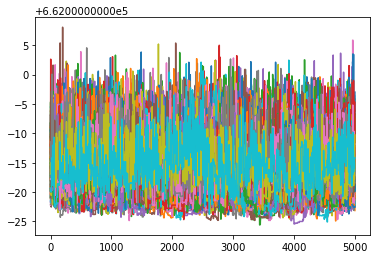
# Verify that the chains have reached a minima
lp = fitter.logpost
fig = plt.plot(-lp)
Check on the final results
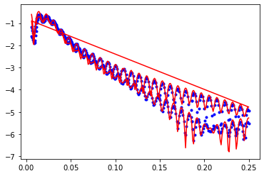
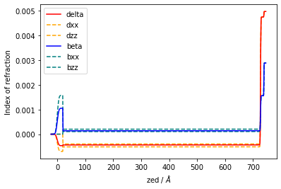
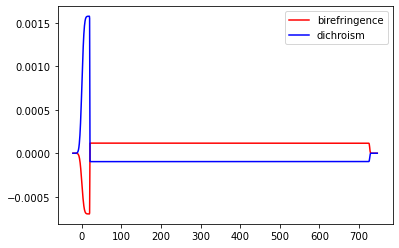
Each objective and structure can now be plotted to look at the final result.
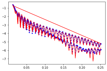
[12]:
obj1 = obj_en1.plot()
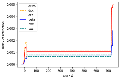
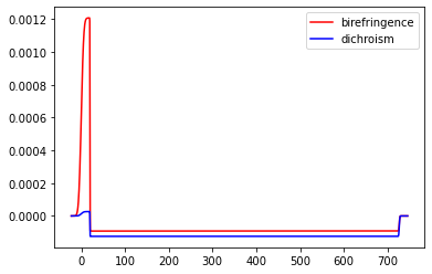
[13]:
struct_en1 = structure_en1.plot(difference=True) # Depth profile w/ orientation
[14]:
obj2 = obj_en2.plot()
[15]:
struct_en2 = structure_en2.plot(difference=True) # Depth profile w/ orientation
[16]:
# Check on the final parameters
# Note that there is only one parameter for the roughness/thickness of each layer.
print(objective.varying_parameters())
________________________________________________________________________________
Parameters:      None
<Parameter:'posa1_surf_thick', value=19.9505 +/- 0.012, bounds=[5.0, 30.0]>
<Parameter:'posa1_surf_xx', value=-0.000698515 +/- 4e-06, bounds=[-0.1, -1e-07]>
<Parameter:'posa1_surf_ixx', value=0.0015763 +/- 2.27e-06, bounds=[0.0, 0.01]>
<Parameter:'posa1_surf_zz', value=-2.02562e-07 +/- 1.24e-07, bounds=[-0.1, -1e-07]>
<Parameter:'posa1_surf_izz', value=5.06237e-08 +/- 6.02e-08, bounds=[0.0, 0.01]>
<Parameter:'posa1_surf_rough', value=4.40916 +/- 0.00994, bounds=[0.5, 20.0]>
<Parameter: 'posa1_thick' , value=706.954 +/- 0.0142, bounds=[400.0, 900.0]>
<Parameter:  'posa1_xx'   , value=-0.000398396 +/- 7.29e-07, bounds=[-0.01, -1e-07]>
<Parameter:  'posa1_ixx'  , value=0.000104594 +/- 2.4e-07, bounds=[0.0, 0.01]>
<Parameter:  'posa1_zz'   , value=-0.000514603 +/- 4.82e-07, bounds=[-0.01, -1e-07]>
<Parameter:  'posa1_izz'  , value=0.000201188 +/- 2.2e-07, bounds=[0.0, 0.01]>
<Parameter: 'posa1_rough' , value=0.200537 +/- 0.000637, bounds=[0.2, 20.0]>
<Parameter: 'SiO2_rough'  , value=1.00031 +/- 0.000391, bounds=[1.0, 10.0]>
<Parameter:'posa2_surf_xx', value=0.00183468 +/- 1.23e-06, bounds=[-0.01, 0.01]>
<Parameter:'posa2_surf_ixx', value=0.000461137 +/- 2.42e-06, bounds=[0.0, 0.01]>
<Parameter:'posa2_surf_zz', value=0.000627185 +/- 9.45e-07, bounds=[-0.01, 0.01]>
<Parameter:'posa2_surf_izz', value=0.000434721 +/- 1.09e-06, bounds=[0.0, 0.01]>
<Parameter:  'posa2_xx'   , value=0.00101304 +/- 5.12e-07, bounds=[-0.01, 0.01]>
<Parameter:  'posa2_ixx'  , value=0.00063915 +/- 3.83e-07, bounds=[0.0, 0.01]>
<Parameter:  'posa2_zz'   , value=0.00110526 +/- 5.17e-07, bounds=[-0.01, 0.01]>
<Parameter:  'posa2_izz'  , value=0.00076358 +/- 3.52e-07, bounds=[0.0, 0.01]>