ALS11012 PRSoXR loader

This tutorial will guide you toward importing your newly aquired p-RSoXR data using the ALS_PRSoXR_Loader. The data can either be exported as a .csv file or the entire dataset can be compiled into an hdf5 file for a more complete meta-data friendly experience.

The first step will be to sort your newly acquired data. The provided utilities draw all files within a single directory and assume they belong to the same reflectivity curve. In the following example, the data has been sorted into directories by sample/polarization/energy.

Loading your data

The following packages are required for loading data

%matplotlib inline
import matplotlib.pyplot as plt
import pathlib
import sys

sys.path.append("../../../src/PyPXR/")
from prsoxr_loader import *

The first step to reduce data with this tool is to create a list that contains a path to each .fits file.

path_s = pathlib.Path('../../../src/PyPXR/example_data/MF201/')
files = list(path_s.glob('*fits'))

files[:5] #Look at the first 5 files.

[WindowsPath('../../../src/PyPXR/example_data/MF201/MFSeries_spol_67235-01744.fits'),
 WindowsPath('../../../src/PyPXR/example_data/MF201/MFSeries_spol_67235-01746.fits'),
 WindowsPath('../../../src/PyPXR/example_data/MF201/MFSeries_spol_67235-01747.fits'),
 WindowsPath('../../../src/PyPXR/example_data/MF201/MFSeries_spol_67235-01748.fits'),
 WindowsPath('../../../src/PyPXR/example_data/MF201/MFSeries_spol_67235-01749.fits')]

Note that the files don’t start at ‘00001’. These have been separated from a longer multiple-sample scan.

The PrsoxrLoader is used to bring the entire dataset into memory.

loader = PrsoxrLoader(files, name='MF201_spol_250eV')

Variables used in reducing the data can be found by printing the new loader object

print(loader)

Sample Name - MF201_spol_250eV
Number of scans - 400
______________________________
Reduction Variables
______________________________
Shutter offset = 0.00389278
Sample Location = 0
Angle Offset = 0.374
Energy Offset = 0
SNR Cutoff = 1.01
______________________________
Image Processing
______________________________
Image X axis = 200
Image Y axis = 200
Image Edge Trim = (5, 5)
Dark Calc Location = LHS
Dizinger Threshold = 10
Dizinger Size = 3

We can note a few things about this dataset:

1. It contains 402 images that need to be reduced

2. The sample was mounted on the top of the sample plate (Sample Location = 0)

3. The Angle Offset is automatically determined to be 0.375

4. A dark frame will be created on the ‘left hand side’ of the image

All other parameteres can be set by the user depending on their prefered settings. See the API for a full list of variables and how they are used in the reduction.

Check individual scans

The PrsoxrLoader.check_spot() utility will allow you to quickly view single scans.

a = loader.check_spot(8, h=40, w=30)

Exposure: 0.00100000004749745
Beam Current: 0.0
Angle Theta: 0.624
T-2T: 0.624
CCD Theta: 1.999
Photon Energy: 249.996035379532
Polarization: 100.0
Higher Order Suppressor: 11.9997548899767
Horizontal Exit Slit Size: 100.0


Processed Variables:
Q: 0.002759278437786943
Specular: 739774
Background: 173296
Signal: 566478
SNR: 4.268846366909796
Beam center (82, 54)

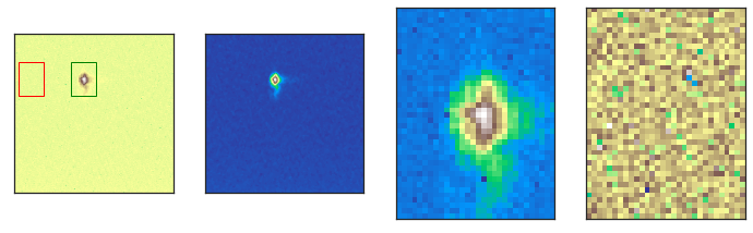
This allows us to get a feel for the beamshape, data quality, and important motor positions. The 4 displayed images are, from left to right:

1. Raw CCD Image, no corrections

2. CCD image passed through a median filter (for locating beamspot)

3. The beamspot determined by the maximum intensity pixel (black box in image 1)

4. The dark frame that will be used for background subtraction (red box in image 1)

The ROI is determined by adjusting the h and w attributes. Adjust the ROI until you fully encompass the beam shape, using PrsoxrLoader.check_spot() to confirm.

Once you have decided on an ROI, you can reduce the data by calling the loader.

refl = loader(h=40, w=30)

The output is a pandas dataframe, we can easily review the data by plotting it. It will also be stored locally in PrsoxrLoader.refl

refl.plot(x='Q', y='R')
plt.yscale('log')

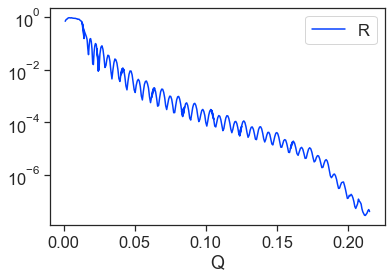
Oh no! Something odd is happening to our data at higher angles! This inflection around Q=0.17 is not a typical behavior of reflectivity, something may have gone wrong in the processing.

Lets review these higher angles using our check_spot function.

a = loader.check_spot(-5, h=40, w=30)

Exposure: 1.0
Beam Current: 0.0
Angle Theta: 59.012
T-2T: 59.012
CCD Theta: 118.0235
Photon Energy: 250.001638213888
Polarization: 100.0
Higher Order Suppressor: 7.50014446251372
Horizontal Exit Slit Size: 1000.0


Processed Variables:
Q: 0.2172012852730185
Specular: 329467
Background: 328126
Signal: 1341
SNR: 1.0040868446877114
Beam center (15, 135)

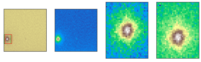
It looks like the beamspot drifts toward the left edge of the image, it is likely tilted on the sample mount. We can see that this causes the light and dark frames to overlap which artifically reduces the intensity. We can adjust the side of the camera that generates a dark frame by updating the PrsoxrLoader.dark_side parameter.

loader.darkside = 'RHS'

Lets check the data again,

refl = loader(h=40, w=30)
refl.plot(x='Q', y='R')
plt.yscale('log')

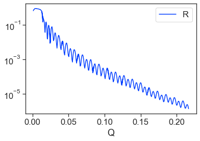
Much better! The dataset looks good and is ready to be exported.

Saving Data

Several options exist for saving data.

• loader.to_csv(path, name, save_meta=True) : This option will save the reflectivity (and meta data) into two .csv. files at the location ‘path’ with the filename ‘name.csv’

• loader.to_hdf5(path, name, save_images=False) : This option will save the reflectivity (and meta data) into a composite .hdf5 file at the location ‘path’ under the filename ‘name.hdf5’

The .csv options provides a much simpler user experience for saving/accessing your data outside of python. The .hdf5 file allows you to compile multiple scans into a single file. Additionally, with save_images=True every processed image is saved under the meta_data umbrella. This will also save the variables used to process the data if you want to review at a later time.

# Saving data in the same folder as this workbook.
loader.to_csv('', 'Samp1_En250_Pol100', save_meta=True) # A .csv file for every energy and polarization
loader.to_hdf5('', 'Samp1', save_images=True) # A single file per sample that sorts by energy and polarization

Your data is now ready to be modeled with PyPXR